Alan A. Lanis, Jr. direct dial: 310.442.8828 jrlanis@bakerlaw.com August 8, 2025 Office of Manufacturing Division of Corporation Finance Securities and Exchange Commission Washington, DC 20549 Attn: Michael Volley and Amit Pande Re: F&G Annuities & Life, Inc. Form 10-K for Fiscal Year Ended December 31, 2024 File No. 001-41490 Messrs. Volley and Pande: On behalf of F&G Annuities & Life, Inc. (the “Company”), we are submitting this letter in response to the comment letter from the staff of the Division of Corporation Finance (the “Staff”) of the Securities and Exchange Commission (the “Commission”) dated July 11, 2025 (the “Comment Letter”), relating to the Company’s Form 10-K, filed with the Commission on February 28, 2025. For the Staff’s convenience, we have repeated below the Staff’s comment in italics, and have followed such comment with the Company’s response. 1. We note your response to prior comment 1. Please explain to us in detail what the MRB Discrete Asset method is and why it is an appropriate methodology to amortize the deferred portion of the changes in fair value of market risk benefits into adjusted net earnings. The MRB Discrete Asset methodology is described in detail below, including illustrative calculations for two consecutive periods. The methodology for amortizing the MRB Discrete Asset is the “constant level basis” methodology as outlined in ASC 944-35-3A, introduced by the FASB in the “Long Duration Targeted Improvements” (LDTI) standards, which were implemented for public-filing companies on 1/1/2023. This methodology is used for amortizing DAC and DAC-like balances, including deferred sales inducements (DSI) as prescribed in ASC 944-30-35-18. MRBs share key characteristics with sales inducements, including: (i) being explicitly identified in the contract at issuance, (ii) representing incremental benefit compared to similar contracts without the feature to attract and attain business, and (iii) being recognized as part of an existing liability. Given these similarities, the MRB Discrete Asset is viewed analogously to a DSI and therefore accounted for in a manner consistent with DSIs. It is an appropriate methodology for amortizing the deferred portion of changes in the MRB fair value because this methodology recognizes the impact of these deferrals over the same period that the MRB is accrued: from contract inception to contract termination. This approach results in amortization that is tied to the MRB balance (via the MRB Discrete Asset), reduces volatility, and provides better matching to the underlying assets that back these liabilities.
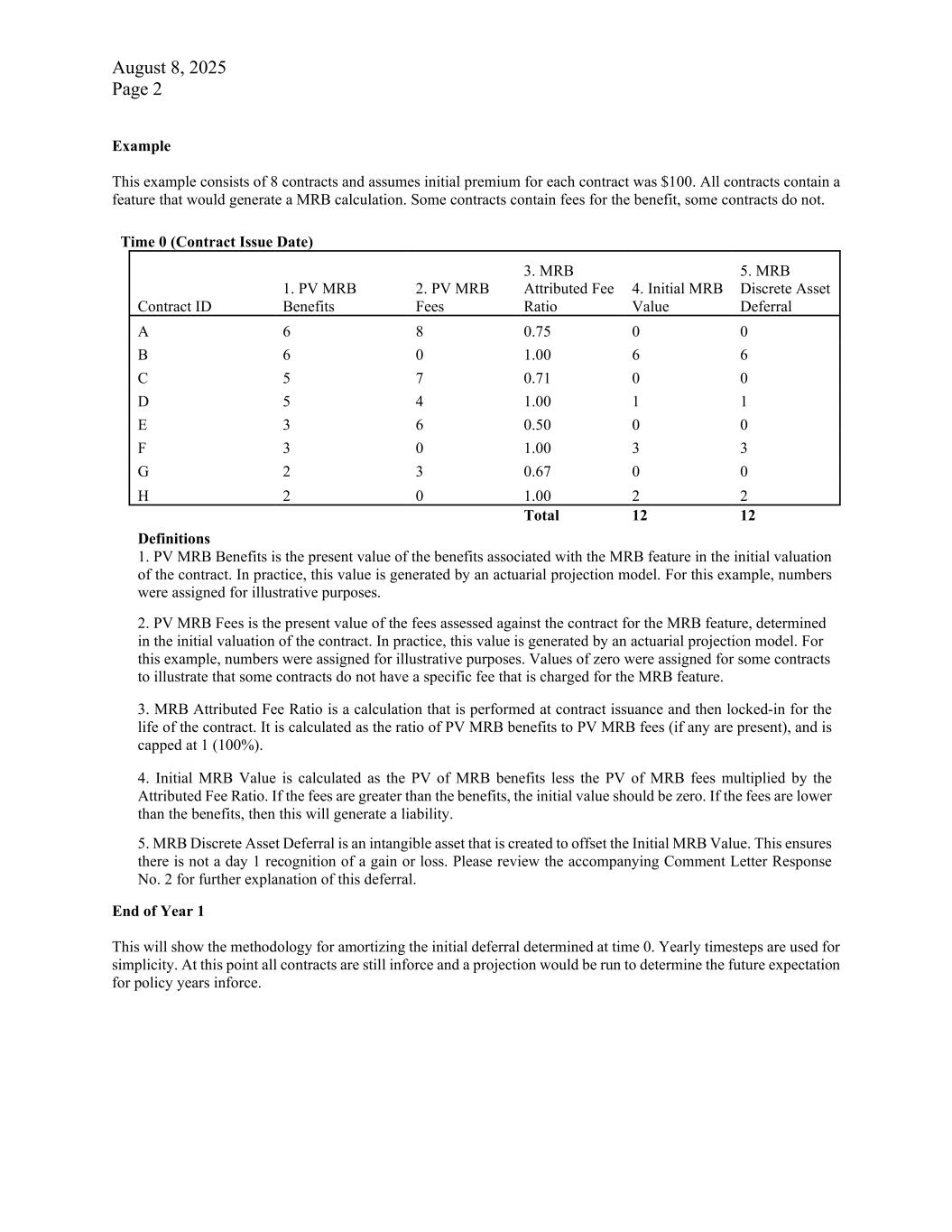
August 8, 2025 Page 2 Example This example consists of 8 contracts and assumes initial premium for each contract was $100. All contracts contain a feature that would generate a MRB calculation. Some contracts contain fees for the benefit, some contracts do not. Time 0 (Contract Issue Date) Contract ID 1. PV MRB Benefits 2. PV MRB Fees 3. MRB Attributed Fee Ratio 4. Initial MRB Value 5. MRB Discrete Asset Deferral A 6 8 0.75 0 0 B 6 0 1.00 6 6 C 5 7 0.71 0 0 D 5 4 1.00 1 1 E 3 6 0.50 0 0 F 3 0 1.00 3 3 G 2 3 0.67 0 0 H 2 0 1.00 2 2 Total 12 12 Definitions 1. PV MRB Benefits is the present value of the benefits associated with the MRB feature in the initial valuation of the contract. In practice, this value is generated by an actuarial projection model. For this example, numbers were assigned for illustrative purposes. 2. PV MRB Fees is the present value of the fees assessed against the contract for the MRB feature, determined in the initial valuation of the contract. In practice, this value is generated by an actuarial projection model. For this example, numbers were assigned for illustrative purposes. Values of zero were assigned for some contracts to illustrate that some contracts do not have a specific fee that is charged for the MRB feature. 3. MRB Attributed Fee Ratio is a calculation that is performed at contract issuance and then locked-in for the life of the contract. It is calculated as the ratio of PV MRB benefits to PV MRB fees (if any are present), and is capped at 1 (100%). 4. Initial MRB Value is calculated as the PV of MRB benefits less the PV of MRB fees multiplied by the Attributed Fee Ratio. If the fees are greater than the benefits, the initial value should be zero. If the fees are lower than the benefits, then this will generate a liability. 5. MRB Discrete Asset Deferral is an intangible asset that is created to offset the Initial MRB Value. This ensures there is not a day 1 recognition of a gain or loss. Please review the accompanying Comment Letter Response No. 2 for further explanation of this deferral. End of Year 1 This will show the methodology for amortizing the initial deferral determined at time 0. Yearly timesteps are used for simplicity. At this point all contracts are still inforce and a projection would be run to determine the future expectation for policy years inforce.
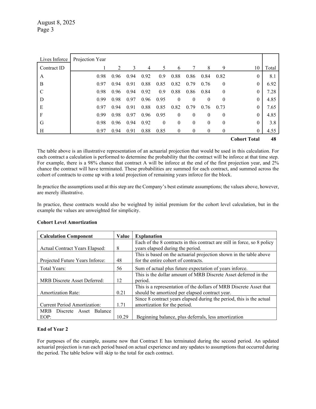
August 8, 2025 Page 3 Lives Inforce Projection Year Contract ID 1 2 3 4 5 6 7 8 9 10 Total A 0.98 0.96 0.94 0.92 0.9 0.88 0.86 0.84 0.82 0 8.1 B 0.97 0.94 0.91 0.88 0.85 0.82 0.79 0.76 0 0 6.92 C 0.98 0.96 0.94 0.92 0.9 0.88 0.86 0.84 0 0 7.28 D 0.99 0.98 0.97 0.96 0.95 0 0 0 0 0 4.85 E 0.97 0.94 0.91 0.88 0.85 0.82 0.79 0.76 0.73 0 7.65 F 0.99 0.98 0.97 0.96 0.95 0 0 0 0 0 4.85 G 0.98 0.96 0.94 0.92 0 0 0 0 0 0 3.8 H 0.97 0.94 0.91 0.88 0.85 0 0 0 0 0 4.55 Cohort Total 48 The table above is an illustrative representation of an actuarial projection that would be used in this calculation. For each contract a calculation is performed to determine the probability that the contract will be inforce at that time step. For example, there is a 98% chance that contract A will be inforce at the end of the first projection year, and 2% chance the contract will have terminated. These probabilities are summed for each contract, and summed across the cohort of contracts to come up with a total projection of remaining years inforce for the block. In practice the assumptions used at this step are the Company’s best estimate assumptions; the values above, however, are merely illustrative. In practice, these contracts would also be weighted by initial premium for the cohort level calculation, but in the example the values are unweighted for simplicity. Cohort Level Amortization Calculation Component Value Explanation Actual Contract Years Elapsed: 8 Each of the 8 contracts in this contract are still in force, so 8 policy years elapsed during the period. Projected Future Years Inforce: 48 This is based on the actuarial projection shown in the table above for the entire cohort of contracts. Total Years: 56 Sum of actual plus future expectation of years inforce. MRB Discrete Asset Deferred: 12 This is the dollar amount of MRB Discrete Asset deferred in the period. Amortization Rate: 0.21 This is a representation of the dollars of MRB Discrete Asset that should be amortized per elapsed contract year. Current Period Amortization: 1.71 Since 8 contract years elapsed during the period, this is the actual amortization for the period. MRB Discrete Asset Balance EOP: 10.29 Beginning balance, plus deferrals, less amortization End of Year 2 For purposes of the example, assume now that Contract E has terminated during the second period. An updated actuarial projection is run each period based on actual experience and any updates to assumptions that occurred during the period. The table below will skip to the total for each contract.
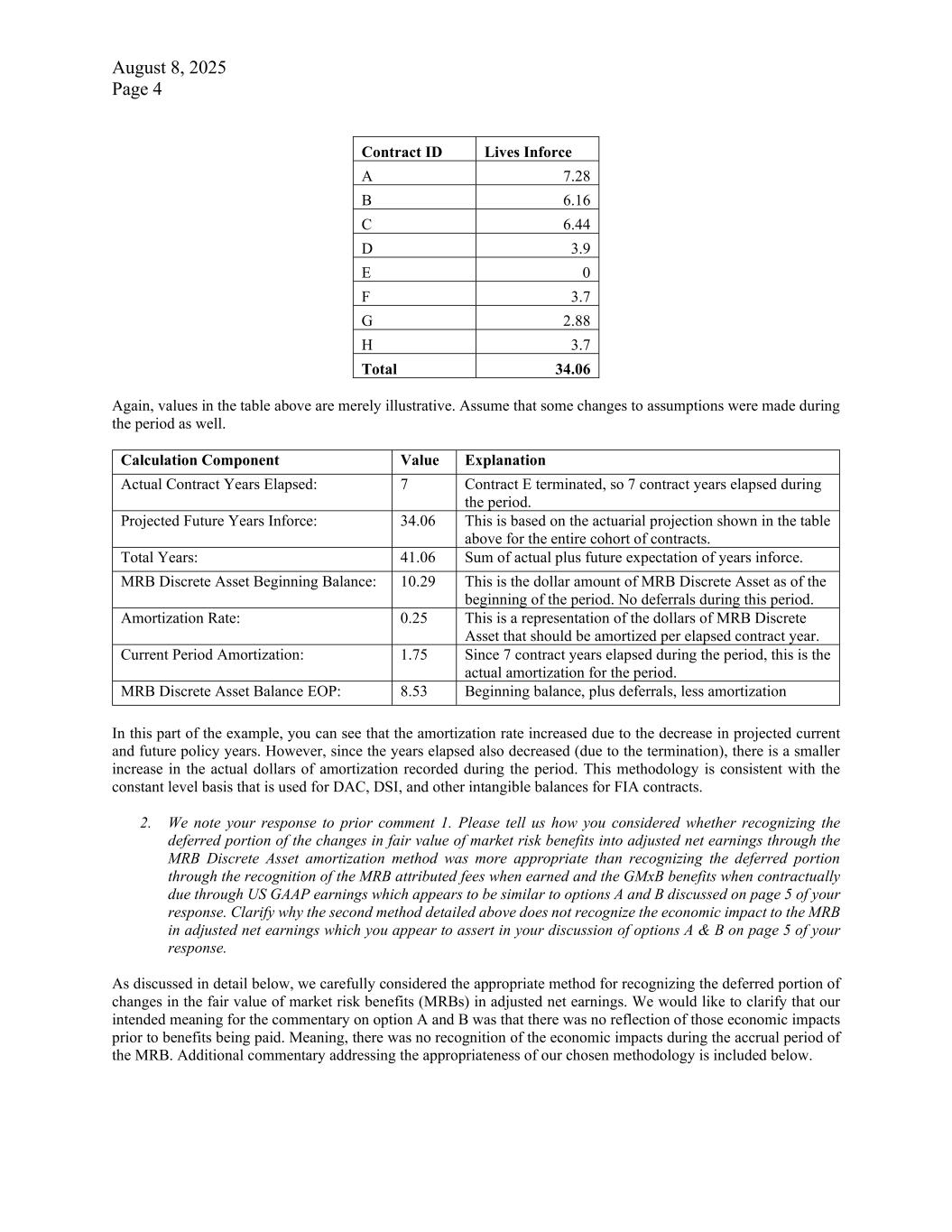
August 8, 2025 Page 4 Contract ID Lives Inforce A 7.28 B 6.16 C 6.44 D 3.9 E 0 F 3.7 G 2.88 H 3.7 Total 34.06 Again, values in the table above are merely illustrative. Assume that some changes to assumptions were made during the period as well. Calculation Component Value Explanation Actual Contract Years Elapsed: 7 Contract E terminated, so 7 contract years elapsed during the period. Projected Future Years Inforce: 34.06 This is based on the actuarial projection shown in the table above for the entire cohort of contracts. Total Years: 41.06 Sum of actual plus future expectation of years inforce. MRB Discrete Asset Beginning Balance: 10.29 This is the dollar amount of MRB Discrete Asset as of the beginning of the period. No deferrals during this period. Amortization Rate: 0.25 This is a representation of the dollars of MRB Discrete Asset that should be amortized per elapsed contract year. Current Period Amortization: 1.75 Since 7 contract years elapsed during the period, this is the actual amortization for the period. MRB Discrete Asset Balance EOP: 8.53 Beginning balance, plus deferrals, less amortization In this part of the example, you can see that the amortization rate increased due to the decrease in projected current and future policy years. However, since the years elapsed also decreased (due to the termination), there is a smaller increase in the actual dollars of amortization recorded during the period. This methodology is consistent with the constant level basis that is used for DAC, DSI, and other intangible balances for FIA contracts. 2. We note your response to prior comment 1. Please tell us how you considered whether recognizing the deferred portion of the changes in fair value of market risk benefits into adjusted net earnings through the MRB Discrete Asset amortization method was more appropriate than recognizing the deferred portion through the recognition of the MRB attributed fees when earned and the GMxB benefits when contractually due through US GAAP earnings which appears to be similar to options A and B discussed on page 5 of your response. Clarify why the second method detailed above does not recognize the economic impact to the MRB in adjusted net earnings which you appear to assert in your discussion of options A & B on page 5 of your response. As discussed in detail below, we carefully considered the appropriate method for recognizing the deferred portion of changes in the fair value of market risk benefits (MRBs) in adjusted net earnings. We would like to clarify that our intended meaning for the commentary on option A and B was that there was no reflection of those economic impacts prior to benefits being paid. Meaning, there was no recognition of the economic impacts during the accrual period of the MRB. Additional commentary addressing the appropriateness of our chosen methodology is included below.
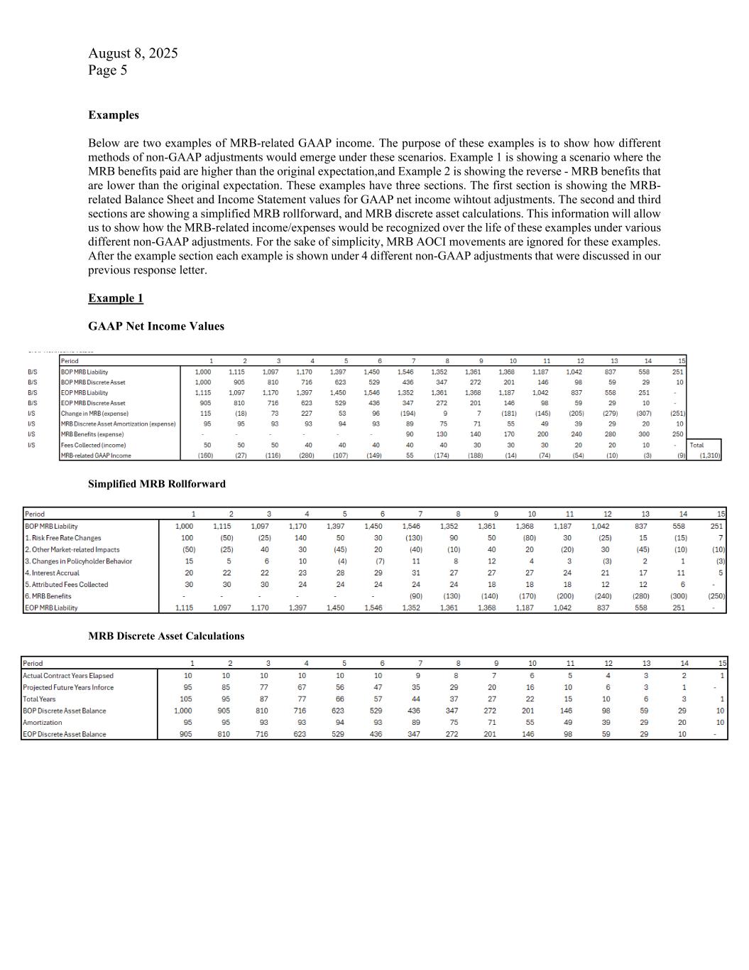
August 8, 2025 Page 5 Examples Below are two examples of MRB-related GAAP income. The purpose of these examples is to show how different methods of non-GAAP adjustments would emerge under these scenarios. Example 1 is showing a scenario where the MRB benefits paid are higher than the original expectation,and Example 2 is showing the reverse - MRB benefits that are lower than the original expectation. These examples have three sections. The first section is showing the MRB- related Balance Sheet and Income Statement values for GAAP net income wihtout adjustments. The second and third sections are showing a simplified MRB rollforward, and MRB discrete asset calculations. This information will allow us to show how the MRB-related income/expenses would be recognized over the life of these examples under various different non-GAAP adjustments. For the sake of simplicity, MRB AOCI movements are ignored for these examples. After the example section each example is shown under 4 different non-GAAP adjustments that were discussed in our previous response letter. Example 1 GAAP Net Income Values Simplified MRB Rollforward MRB Discrete Asset Calculations
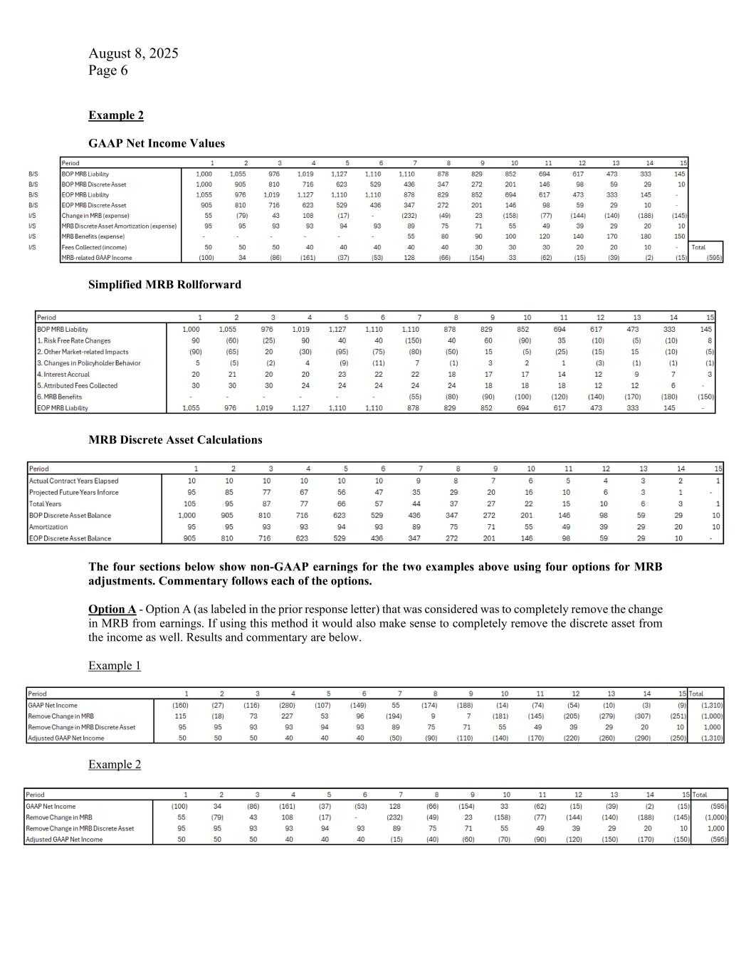
August 8, 2025 Page 6 Example 2 GAAP Net Income Values Simplified MRB Rollforward MRB Discrete Asset Calculations The four sections below show non-GAAP earnings for the two examples above using four options for MRB adjustments. Commentary follows each of the options. Option A - Option A (as labeled in the prior response letter) that was considered was to completely remove the change in MRB from earnings. If using this method it would also make sense to completely remove the discrete asset from the income as well. Results and commentary are below. Example 1 Example 2
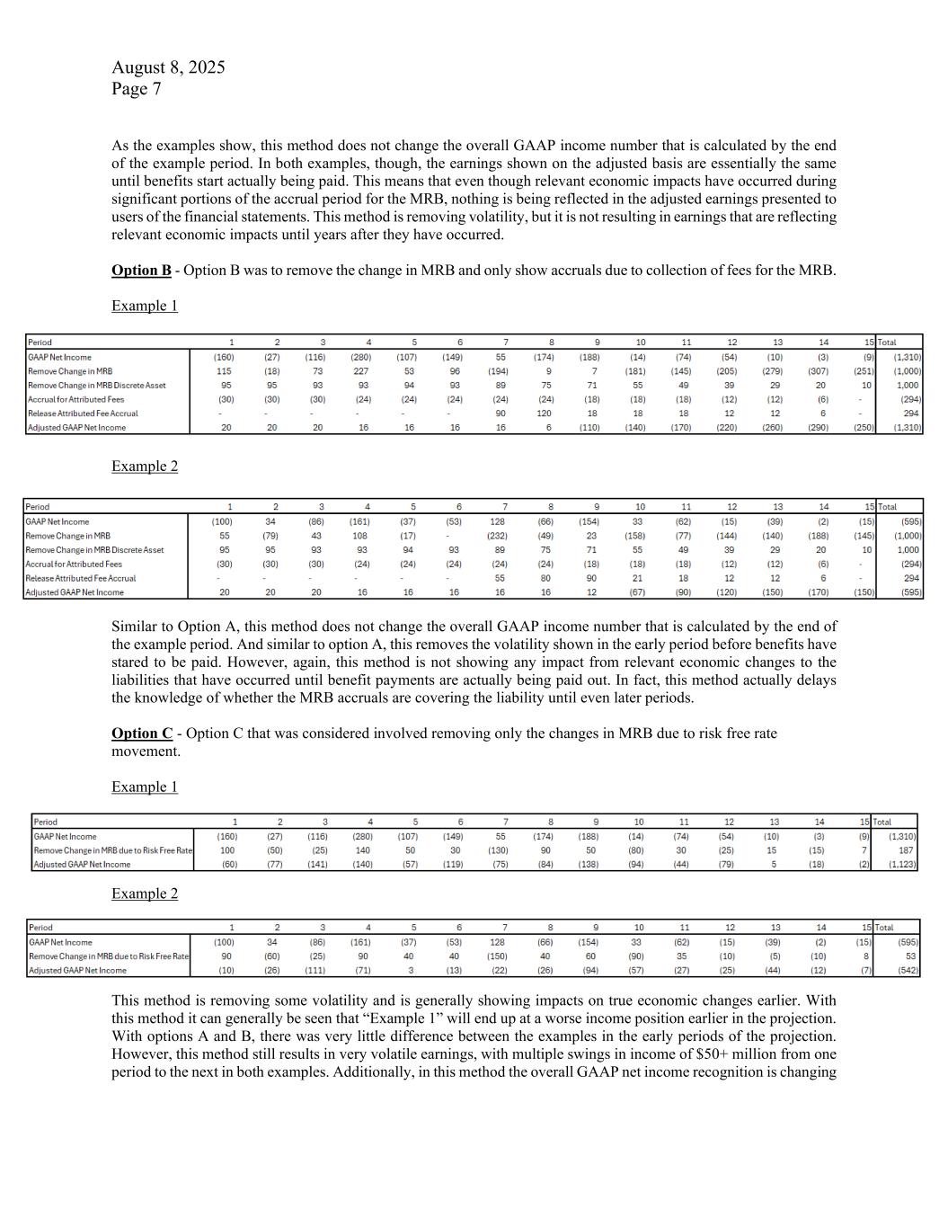
August 8, 2025 Page 7 As the examples show, this method does not change the overall GAAP income number that is calculated by the end of the example period. In both examples, though, the earnings shown on the adjusted basis are essentially the same until benefits start actually being paid. This means that even though relevant economic impacts have occurred during significant portions of the accrual period for the MRB, nothing is being reflected in the adjusted earnings presented to users of the financial statements. This method is removing volatility, but it is not resulting in earnings that are reflecting relevant economic impacts until years after they have occurred. Option B - Option B was to remove the change in MRB and only show accruals due to collection of fees for the MRB. Example 1 Example 2 Similar to Option A, this method does not change the overall GAAP income number that is calculated by the end of the example period. And similar to option A, this removes the volatility shown in the early period before benefits have stared to be paid. However, again, this method is not showing any impact from relevant economic changes to the liabilities that have occurred until benefit payments are actually being paid out. In fact, this method actually delays the knowledge of whether the MRB accruals are covering the liability until even later periods. Option C - Option C that was considered involved removing only the changes in MRB due to risk free rate movement. Example 1 Example 2 This method is removing some volatility and is generally showing impacts on true economic changes earlier. With this method it can generally be seen that “Example 1” will end up at a worse income position earlier in the projection. With options A and B, there was very little difference between the examples in the early periods of the projection. However, this method still results in very volatile earnings, with multiple swings in income of $50+ million from one period to the next in both examples. Additionally, in this method the overall GAAP net income recognition is changing
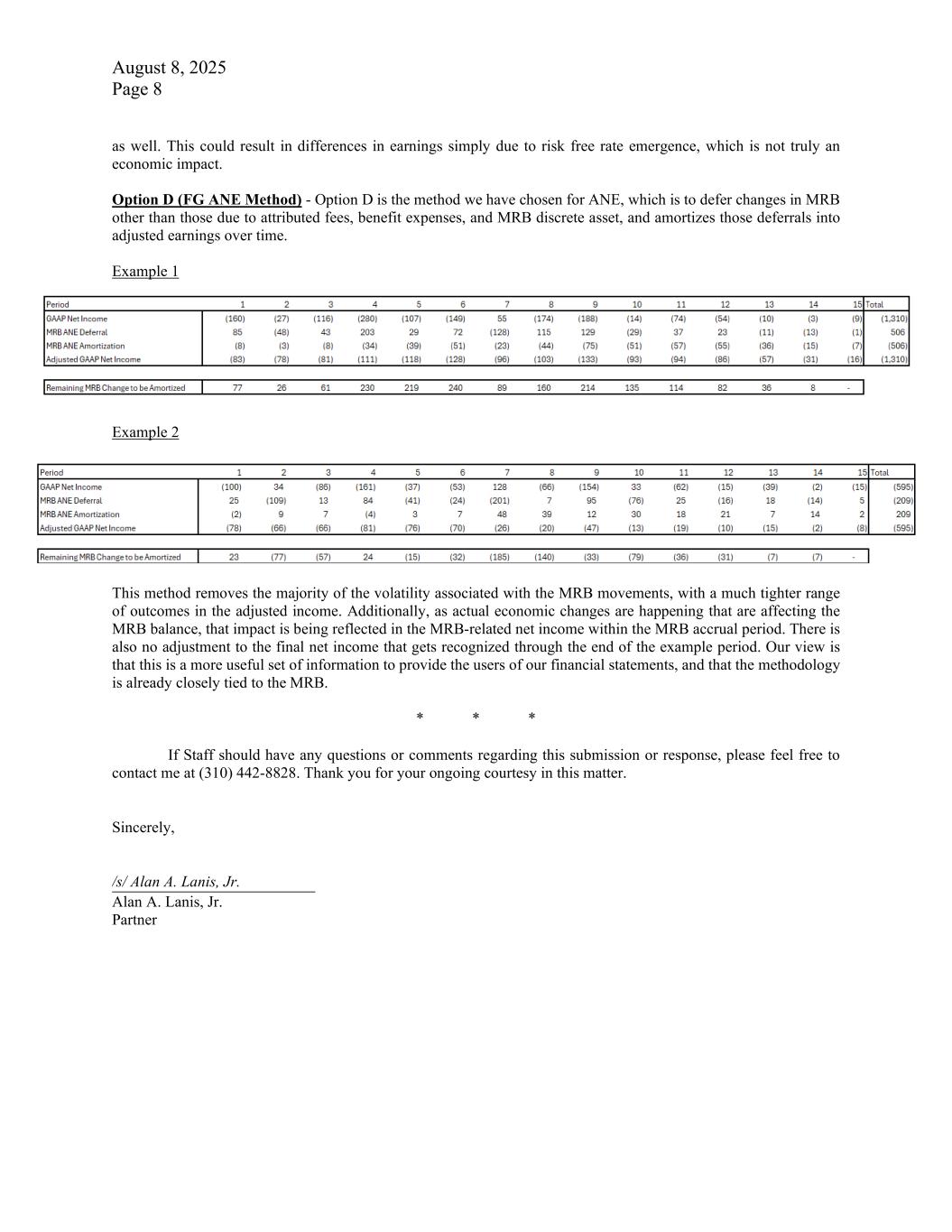
August 8, 2025 Page 8 as well. This could result in differences in earnings simply due to risk free rate emergence, which is not truly an economic impact. Option D (FG ANE Method) - Option D is the method we have chosen for ANE, which is to defer changes in MRB other than those due to attributed fees, benefit expenses, and MRB discrete asset, and amortizes those deferrals into adjusted earnings over time. Example 1 Example 2 This method removes the majority of the volatility associated with the MRB movements, with a much tighter range of outcomes in the adjusted income. Additionally, as actual economic changes are happening that are affecting the MRB balance, that impact is being reflected in the MRB-related net income within the MRB accrual period. There is also no adjustment to the final net income that gets recognized through the end of the example period. Our view is that this is a more useful set of information to provide the users of our financial statements, and that the methodology is already closely tied to the MRB. * * * If Staff should have any questions or comments regarding this submission or response, please feel free to contact me at (310) 442-8828. Thank you for your ongoing courtesy in this matter. Sincerely, /s/ Alan A. Lanis, Jr. Alan A. Lanis, Jr. Partner